
A more formal analysis of the derivation and
meaning of the CMB anisotropy vectors
by Dr. Alec MacAndrew (02/13/2015)
In “Yes, the CMB Misalignments Are a Problem for the New Geocentrists“, we have explained that the CMB anisotropy vectors carry no position information and do not point directly, or even approximately, at the Earth, as the neo-geocentrists claim. We recognise that most people reading that article will be satisfied with the explanations we have already given, but of course the nature and interpretation of these vectors is based on their mathematical definition within the physical framework. So for those of you who have the interest, we have included this second article, which takes a more formal approach to showing that the fundamental proposition of the Principle movie and much of the geocentrists’ recent propaganda efforts – which is that the CMB anomalies are evidence for the central (or near-central or special) location of the Earth in the Universe – are based on an erroneous interpretation of the physics and data analysis of the CMB.
CMB anisotropy means that the temperature of the CMB is different depending on which direction we look. Measurements carried out by a wide range of satellite and balloon missions show that it varies a tiny amount all over the sky (the intrinsic component is about one part in 100,000). This anisotropy is predicted very accurately by the standard inflationary ΛCDM model as described in my recent article on the CMB [1]. The anisotropy map is therefore a function of the CMB temperature on the spherical surface of last scattering. The surface of last scattering is where the CMB photons first started propagating towards the Earth. The Earth is then, by definition, at the centre of the surface of last scattering and the CMB is localised on the surface, because the photons have all taken the same time to travel from the surface to the Earth. Since the CMB pervades the Universe, the surface of last scattering or the sphere of the CMB is always centred on the observer, wherever she is.
Representation of the CMB as spherical harmonics
As far as this analysis goes, we are not interested in the absolute temperature of the CMB, but in its variation with direction, so we define a variable on spherical co-ordinates:

where ΔT is the CMB anisotropy on the sphere, T the temperature in direction (θ, Φ) and <T> the average temperature. Since ΔT is defined on a sphere, we can decompose the CMB anisotropy into a series of spherical harmonics or multipoles (this process is analogous to the much better known idea of a Fourier series in which the function of a variable is decomposed into the sum of an infinite harmonic series of sinusoids). The mathematics is absolutely standard and can be found in numerous text books and websites.[14] We decompose the anisotropy signal into an infinite series of multipoles (l, m):

Where the
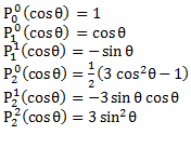
 and Plm are the associated Legendre polynomials [2] [3]. So according to Eq. 2 and Eq. 3, the entire CMB anisotropy is the sum of an infinite series of independent multipoles of order l, where l defines the angular size and number of lobes of each multipole so that: l=1 is the dipole with two lobes, one warmer, one cooler, and each lobe covers half the sky; l=2 is the quadrupole with four lobes, two warmer, two cooler and each lobe covers a quarter of the sky; l=3 is the octopole with eight lobes etc. The index, m, which ranges from –l to +l, determines how the warm and cool lobes are interleaved on the sky.
So, for example, for the dipole, the l=1, m=0 component has the warm and cool lobes centred on the polar-axis of the coordinate system; the l=1, m=1 component has the warm and cool lobes at θ = 0 and 180 respectively, Φ=90; and the l=1, m=-1 component has the warm and cool lobes rotated by 90° in with respect to l=1, m=1 component. In general the –m components are the same as the +m components rotated by 90°/m. We are concerned in this article only with the dipole, quadrupole and octopole (l=1,2,3) [4], and Figure 1 illustrates the components of the multipoles up to l=4
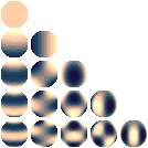 Fig 1. “Rotating spherical harmonics”. Real (Laplace) spherical harmonics for l= 0 to 4 (top to bottom) and m = 0 to 4 (left to right). Licensed under CC BY-SA 3.0 via Wikimedia Commons
A similar but visually more exciting graphic can also be found on-line [5].
The well-known CMB anisotropy power spectrum is derived from the coefficients alm of the multipole decomposition in Eq. 2 by:
 The temperature fluctuation is usually plotted as l(l+1)Cl/2π:
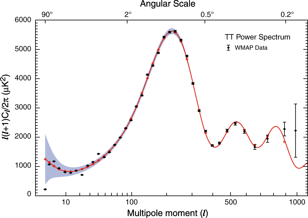
Fig 2. The three-year WMAP CMB power spectrum. The vertical axis represents the amount of anisotropy and the horizontal axis represents the scale, with large scale modes towards the left and fine scale modes to the right. The theoretical prediction of the standard ΛCDM model is the red curve and the experimental data are the black points with error bars. Source NASA/WMAP Science Team#
Directions associated with the multipoles
So, let’s look at the various means that have been used to define directions associated with individual multipoles.
Multipole vectors
We’ll begin with the definition and method of Copi et al [6]. Each multipole can be defined as follows, either as a spherical harmonic or in terms of multipole vectors:
 Thus the CMB anisotropy in the multipole vector expansion depends on a scalar Al and the product of l unit vectors û(l , i) where i =1,…,l (the multipole vectors) and where ê (θ, Φ) is a unit vector in the (θ, Φ) direction. The unit vectors û(l , i) are known as the multipole vectors. The term τl is included to make the expression traceless and need not concern us. Since we are considering only l=1,2,3 (the dipole, quadrupole and octopole), we are considering multipoles with one, two and three multipole vectors respectively. This multipole vector representation of a field on a sphere has been shown to be identical to that developed by James Clerk Maxwell in 1891 [6]. An algorithm for extracting the multipole vectors from the CMB data has been presented by Copi et al [7].
Copi et al, and Abramo et al say this about the multipole vectors:
These unit vectors v(ℓ,j) are only defined up to a sign (and are thus “headless vectors”), as a change in sign of the vector can always be absorbed by the scalar Al We have chosen the convention that multipole vectors point in the northern Galactic hemisphere, although when plotting them we often instead show the southern counterpart for clarity. [6]
This “reflection symmetry” implies that the multipole vectors define only directions , hence they are “vectors without arrowheads” living on the half-sphere with antipodal points identified [8] [My emphasis]
Both papers make it clear that the multipole vectors define only directions of CMB features on the spherical surface of last scattering and do not carry information about the position of the Earth (or any object in the Universe). Indeed, that is obvious from the fact that the entire analysis is carried out in spherical co-ordinates (θ, Φ) (and not in (r, θ, Φ)). The vectors identify directions of CMB features and they are a function of (θ, Φ) and so are unable to define positions in R3. The vectors necessarily originate at the point of observation, and therefore it can be said that all the CMB vectors (including but not limited to the multipole vectors) “pass through” the Earth because that is where we are [9]. A hypothetical alien 100 million light years away doing these measurements and this analysis would acknowledge that all the multipole vectors originate at his location. Note also that the vectors are only defined up to a sign – we can’t distinguish between û(l , i) and – û(l , i) – in other words, they define the orientation of a plane, but they do not resolve the +/- direction ambiguity. As we’ll see, this sign degeneracy is true for all the different vectors used to assess alignments of the CMB features (because they are the vector representations of planes). Finally, the multipole vectors are unit vectors, providing further proof, if that were needed, that they do not define positions in R3.
Normal or area vectors
The multipole vectors are not the most useful way to test for anomalous alignments in the CMB (note also that they don’t align anywhere near each other and apart from the dipole vector they don’t align anywhere near the equinox or ecliptic either) and so Copi et al define the area or normal vectors:
![]()
By the rules of the vector product we can see that an area vector is normal to the plane in which pairs of the multipole vectors lie, and its amplitude (on the interval 0 to 1) is sin(α) where α is the angle between the multipole vector pairs. We can immediately see that, since the area vectors depend on pairs of multipole vectors, the number of area vectors for each multipole is given by n=l (l-1)/2. So the dipole, having only one multipole vector has no area vector; the quadrupole has two multipole vectors which define one plane and one area vector; and the octopole has three multipole vectors, and therefore three pairs which define three planes and three area vectors.
Note that since the area vectors depend solely on the multipole vectors, then the area vectors also carry no position information, being determined purely by angular spherical co-ordinates. They, like the multipole vectors, originate at the point of observation by definition and they also are defined only up to a sign. They do not carry information about the position of the Earth (or any object in the Universe).
In references [[6], [7], [10]] Copi et al analyse the alignment of the area vectors of the quadrupole and the octopole with the dipole, ecliptic plane and the equinox. See for example figure 3.
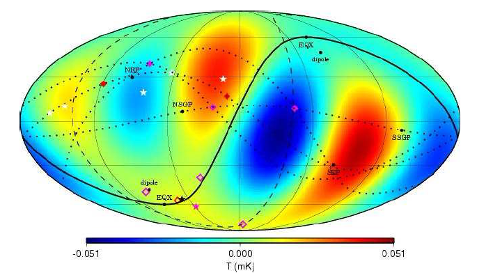
Fig 3. The l=2 and 3 alignments from Tegmark 2003 cleaned maps [11]. The solid line is the ecliptic plane, the equinoxes (EQX), the dipole and the ecliptic poles (NEP and SEP) are marked. The solid red diamonds are the two quadrupole vectors, the solid pink diamonds are the three octopole vectors. The open red diamond is the quadrupole area vector and MAMD vector (see below). The open pink diamonds are the three octopole area vectors and the pink star is the octopole MAMD vector. Figure from reference [6]
MAMD
Since there are three area vectors for the octopole (and increasingly more with increasing multipole: six for l=4, 10 for l=5 etc), then cosmologists sought an alternative measure for assessing the alignment of the multipoles. The method, first developed by de Oliveira-Costa et al [12], is to find the vector or axis n around which the angular momentum dispersion:

is maximised (MAMD) for each multipole l, where alm are the spherical harmonic coefficients of Eq. 2, measured in a co-ordinate system rotated so that the z- axis is in the n direction. These are the MAMD vectors. This method results in one vector per multipole. The quadrupole MAMD vector can be shown to be in the same direction (under certain conditions that we needn’t go into here) as the quadrupole area vector, and the octopole MAMD vector lies near to the cluster of octopole area vectors. The MAMD vectors are the single measure used by the Planck team to assess the alignment of the multipoles. The Planck team in their major paper on isotropy and statistics of the CMB says this about these vectors:
This definition of the multipole orientation has been devised for planar multipoles and is simply the direction perpendicular to the plane in which most of the power of the multipole lies. It is thus intuitive and easy to use. Note that the value of the statistic in Eq. (26) [our Eq. 7] is the same for −n as for n, i.e., the multipole orientation is only defined up to a sign. [13]
“The plane in which most of the power of the multipole lies” is the plane where the sum of the squares of the absolute values of the multipole coefficients is maximized; and we can think of this as being defined by an axis around which the anisotropy variations of the CMB temperature is greatest. It is immediately clear that the plane passes through the point of observation by definition, as does the axis n. As we have seen before for multipole and area vectors, the sign of the MAMD vector is not defined, which means it encodes an orientation and has sign degeneracy; and again it carries no position information.
The anomalous alignments
The various statistics described above have been used to assess the anomalous alignments of the dipole, quadrupole and octopole with themselves and the Earth’s ecliptic plane and equinox in multiple scientific papers. The alignments appear to be anomalous because the various features align more closely (ie the angles between the vectors are smaller) than would be expected if the features are independent. It’s not the purpose of this article to discuss the anomalous alignments per se – that has been done elsewhere – but to show that the various vectors and planes discussed by cosmologists in this context carry no position information and so cannot, as the neo-geocentrists claim, distinguish the location of the Earth in the Universe exactly nor approximately, nor indeed, at all.
Conclusion
For many years, the neo-geocentrists have been claiming that the alignments of the low-l multipoles with one another and with local features such as the ecliptic plane and the equinoxes is evidence for the central (or near-central, or special) location of the Earth in the Universe – indeed, as we have seen in this article “The CMB Alignment Challenge”, they have all made claims that the features point directly at the Earth.
In this somewhat more technical article, we have shown that the various vectors and planes do not carry any position information, and moreover, according to their definition, they cannot. Furthermore, we have seen that all the vectors derived from the CMB data have their origin at the point of observation, in our case the Earth9, by definition. They cannot, as the neo-geocentrists claim, distinguish the Earth directly or approximately (or, indeed, at all).
Since these conclusions are inherent to the mathematical definitions of the various vectors, it follows that the geocentrists’ claims that the CMB anomalies are evidence for a central or special location of the Earth cannot be justified on this evidence.
[1] https://www.geocentrismdebunked.org/the-cmb-and-geocentrism/
[2] http://mathworld.wolfram.com/AssociatedLegendrePolynomial.html
[3] The first few associated Legendre polynomials which are the ones that concern us are:
 See, for example: http://mathworld.wolfram.com/AssociatedLegendrePolynomial.html
[4] Although this article discusses the multipoles only up to l=3 explicitly, its main point, that the vectors carry no position information, stands for all multipoles
[5] http://find.spa.umn.edu/~pryke/logbook/20000922/
[6] Copi et al, On the large-angle anomalies of the microwave sky, http://arxiv.org/pdf/astro-ph/0508047v1.pdf
[7] Copi, Huterer and Starkman, Multipole Vectors–a new representation of the CMB sky and evidence for statistical anisotropy or non-Gaussianity at 2<=l<=8, http://arxiv.org/pdf/astro-ph/0310511v2.pdf
[8] Abramo et al, Alignment tests for low-CMB multipoles, http://arxiv.org/pdf/astro-ph/0604346.pdf
[9] This is an approximation: I’m ignoring the fact that the WMAP and Planck satellites were located not at the Earth but at the Earth-Sun Lagrange point L2, almost a million miles from Earth, and the annual modulation of the orbit of L2 around the Solar System barycentre was averaged out in the data, making the barycentre the origin of observation
[10] Copi et al, Large-scale alignments from WMAP and Planck, http://arxiv.org/pdf/1311.4562.pdf
[11] Tegmark et al, A high resolution foreground cleaned CMB map from WMAP, http://arxiv.org/abs/astro-ph/0302496
[12] de Oliveira-Costa et al, The significance of the largest scale CMB fluctuations in WMAP, http://arxiv.org/pdf/astro-ph/
[13] Planck Team, Planck 2013 results. XXIII. Isotropy and statistics of the CMB, http://arxiv.org/pdf/1303.5083v3.pdf
[14] See for example: http://www.roe.ac.uk/ifa/postgrad/pedagogy/2006_tojeiro.pdf and http://mathworld.wolfram.com/SphericalHarmonic.html. Also reference [7] above